survivalROC
A prognostic marker is only useful if it separates patients who will have an event from patients who will not. For a yes/no outcome, the ROC curve and its area (AUC) measure that. Survival data add two problems: The outcome depends on when you ask, and some patients are censored before you can know.
In 2000, Heagerty, Lumley and Pepe published the time-dependent ROC curve, which answers the question at a chosen time point: Of the patients who died by year 2, how many did the marker flag, and of those still alive, how many did it flag wrongly? Their R package, survivalROC, has been the standard implementation since.
It offers two estimators through one function, survivalROC():
- KM. A Kaplan-Meier estimate among the patients above each cut-off.
- NNE. A nearest-neighbour estimate that smooths over patients with similar marker values. It guarantees a curve that never turns back on itself, which the KM version does not.
A second function, survivalROC.C(), runs the NNE estimate in compiled C.
People use it in a few recurring ways:
- To report a signature. “The 3-year AUC of our risk score was 0.78” in a prognostic-model paper is very often a survivalROC number.
- To screen markers. Compute the AUC for every gene, protein or variable, then rank them.
- To put error bars on an AUC. Recompute it on hundreds or thousands of bootstrap resamples.
- To compare time points. Repeat the calculation at 1, 3 and 5 years.
The last three multiply the number of calls, and that is where the trouble starts.
NbClust
Clustering methods need to be told how many groups to find. There is no single right way to choose that number, so statisticians have proposed dozens of indices, each scoring a candidate number of clusters in a different way.
NbClust (Charrad, Ghazzali, Boiteau and Niknafs, 2014) puts 30 of those indices behind one function call. You give it a data matrix, a clustering method and a range such as 2 to 10 clusters. It computes every index for every candidate, reports which number each index prefers, and returns the majority vote.
People use it in a few recurring ways:
- To justify a number of clusters. “The optimal number of clusters was determined with NbClust” is a standard methods sentence in papers that subtype patients, tumours, cells or survey respondents.
- To compare clustering settings. Run it once per distance and linkage method and see where the indices agree.
- To check stability. Run it again on resampled data and see whether the vote holds.
It has two modes that matter here:
index = "all"computes 26 indices. This is the default and what most people run.index = "alllong"computes all 30. The four extra indices (Gap, Gamma, Gplus and Tau) are left out of the default mode.
Run time grows much faster than the data
We framed both tasks as a speedup problem. A faster tool that changes published numbers in the third decimal place would not be adopted, and should not be.
survivalROC
One call on 161 patients takes a fraction of a second. But the cost of a call grows with the cube of the number of patients. Double the cohort and the wait is eight times longer.
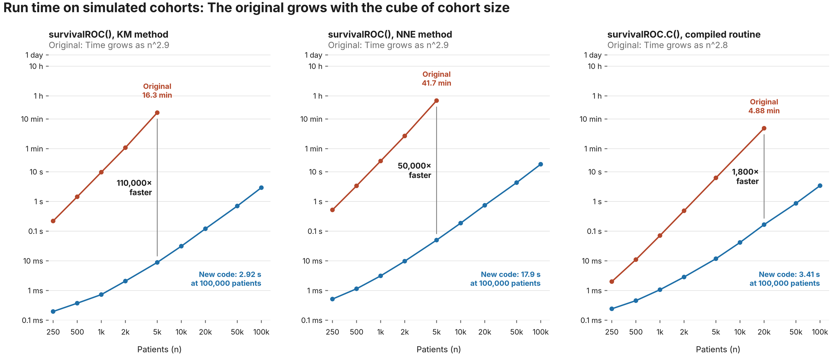
On a simulated cohort of 5,000 patients, one call takes 16 minutes with the KM method and 42 minutes with the NNE method. The compiled routine is faster but follows the same curve: 6 seconds at 5,000 patients and 5 minutes at 20,000.
So the package is fine for one curve on one small cohort and impractical for:
- A marker screen across a transcriptome
- Bootstrap intervals on a cohort of a few thousand
- Any registry, biobank or national survey
NbClust: The fourth power of the data
A profile of NbClust shows the time is concentrated. In the default mode, four groups of internal functions take about 94% of it. In the 30-index mode, one function takes 98%: The one that computes Gamma, Gplus and Tau.
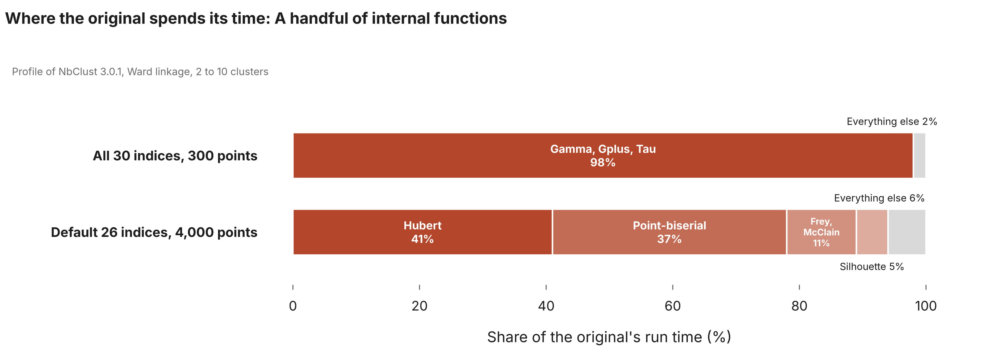
That function compares every within-cluster distance with every between-cluster distance. The number of distances grows with the square of the number of observations, so the number of comparisons grows with the fourth power. Double the data and the wait is sixteen times longer.
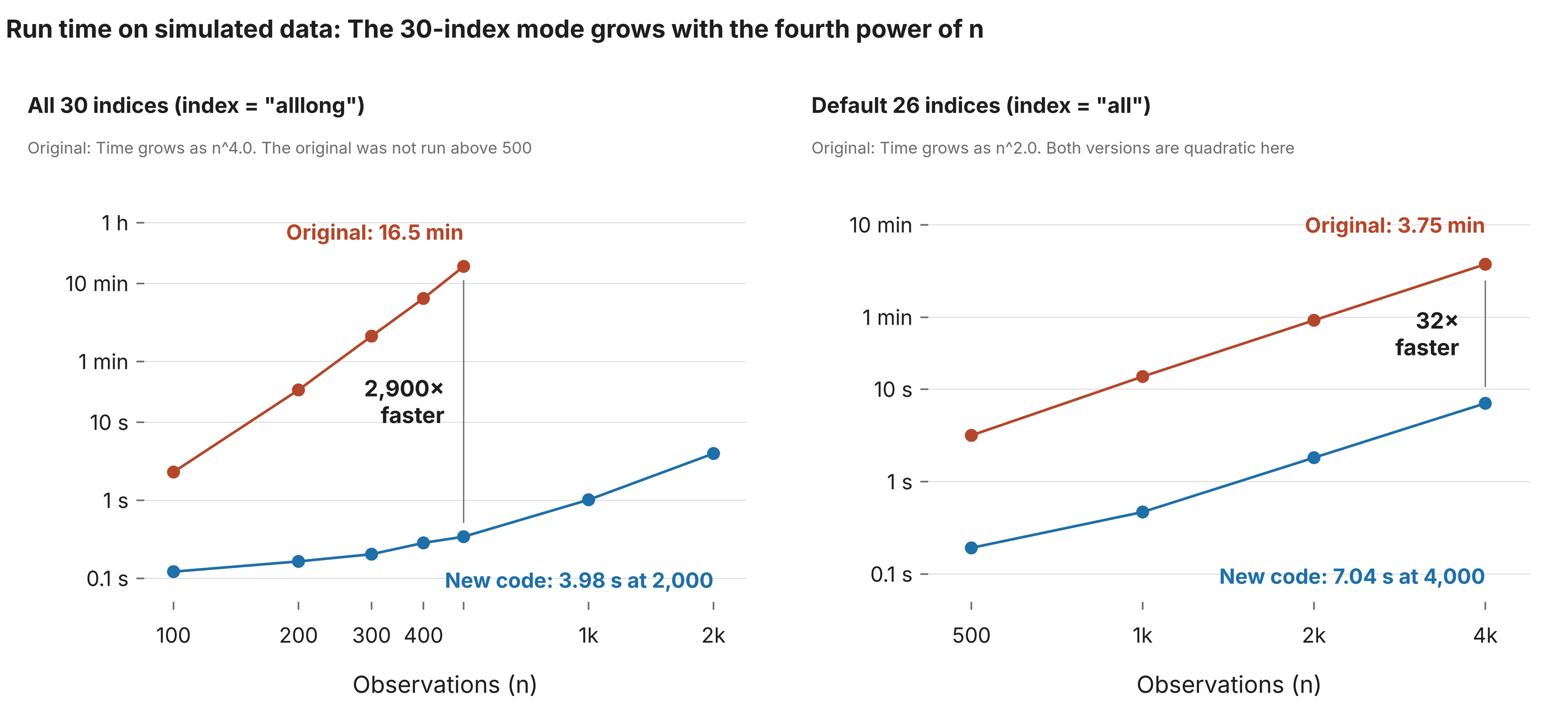
On simulated data, the 30-index mode takes 2.3 seconds for 100 observations and 16.5 minutes for 500. The default mode is better behaved: It grows with the square of the data, which is unavoidable for anything built on a distance matrix, but it carries a large constant. At 4,000 observations it takes 3.75 minutes.
So NbClust is quick for a small study and impractical for:
- All 30 indices on more than a few hundred observations
- Any repeated use, such as resampling or a sweep over clustering settings
- Cohorts in the thousands, even in the default mode
The solution
survivalROC (Faster Survival Analysis)
The Old Problem: In the original code, for every single time cutoff and every event, it re-analyzed every single patient from scratch. As a result, when datasets got larger, the software slowed down dramatically.
The Solution: The new version is faster because it avoids repeating work:
- One-time sorting: It puts the patients in order by time right at the start.
- Efficient loops: For the Kaplan-Meier (KM) method, it only looks through the patients once, updating the results as each death occurs.
- Neighbor tracking: For the Nearest Neighbor (NNE) method, it keeps a running list of neighboring patients. Instead of building a brand-new list for every patient, it just adds or removes a few neighbors as it moves along.
- Exact math: It performs the math using the exact same numbers and in the exact same sequence as before. Because of this, the new results match the old ones 100% identically down to every last digit (they aren’t just close estimates).
NbClust (Faster Cluster Analysis)
The Old Problem: In the original code, it compared items one pair at a time and frequently re-calculated the exact same results multiple times.
The Solution: The new version speeds things up in three smart ways:
- Smart lookups: For certain indices (Gamma, Gplus, and Tau), it sorts the distances between clusters just once. Instead of comparing every pair, it simply checks where a distance sits in that pre-sorted list.
- Compiled speed: For other slow calculations, it uses faster compiled code to run the math, while keeping the steps in the exact same order.
- No repeats (Caching): If the software needs the same result more than once, it calculates it a single time and saves it for reuse.
Technical specifics
survivalROC
Let n be the number of patients, c the number of cut-offs (by default every distinct marker value), d the number of distinct event times before the prediction time, and w the number of patients in a neighbourhood.
| Original | New | |
|---|---|---|
survivalROC(), KM | For each cut-off, for each event time, scan all patients: c × d × n | One pass in time order; each patient updates a running count for the cut-offs below its marker value: At most n × c integer updates, one multiply per death per cut-off |
survivalROC(), NNE | For each marker value, sort all differences, then for each event time scan all patients: c × (n log n + d × n) | A sorted member list slides along the marker axis; each Kaplan-Meier product visits only its members: c × w |
survivalROC.C() | For each marker value, for each event time, scan the window: c × d × w | The same sliding list: c × w, plus c² plain additions for the final sums |
Three details make bit-identity possible:
- Skipped factors are exactly 1. The original multiplies by (1 − deaths/at-risk) at every event time. Where a subgroup has no death, that factor is exactly 1.0, so leaving it out changes nothing. The new code only visits times where the subgroup has a death, and multiplies in the same order.
- Neighbourhoods are contiguous. Every neighbourhood rule in the package selects a run of consecutive marker ranks. The boundaries are found with the original’s own floating-point comparisons, so ties and rounding fall the same way.
- Sums keep R’s order and precision. The last step adds survival estimates over all patients above each cut-off. R’s
sum()accumulates in extended precision in data order. The new code keeps one extended-precision accumulator per cut-off and feeds them in the same order.
The result is a small R package, survivalROCfast, with about 360 lines of C and 240 lines of R. It exports survivalROC() and survivalROC.C() with the original arguments and return values, so library(survivalROCfast) in place of library(survivalROC) is the whole migration.
NbClust
Let n be the number of observations and N = n(n − 1)/2 the number of pairwise distances. For a partition, each distance is either within a cluster or between clusters.
| Index or step | Original | New |
|---|---|---|
| Gamma, Gplus, Tau | For each within-cluster distance, one vectorised comparison against all between-cluster distances: About N² / 4 comparisons, repeated three times per number of clusters | Sort the between-cluster distances once, then two binary searches per within-cluster distance: About N log N operations, done once |
| Hubert, point-biserial | Scalar R loops over all N pairs | The same loop in C, with identical terms in identical order |
| Frey, McClain | Rebuild the within and between distance vectors by growing R vectors, twice per number of clusters | Build each vector once in C in the original order and keep it for the next number of clusters |
| Silhouette | R loop over observations with a submatrix sum per cluster | One pass per observation with one extended-precision accumulator per cluster |
| SD, SDbw, D index | Triple scalar R loops over clusters, variables and observations | The same arithmetic in C |
| Gap | Cluster the simulated reference data again for every replicate and every number of clusters (about 90 times) | The reference data never change (see the defects below), so cluster them once |
| Repeated calls | Some results are recomputed up to seven times per number of clusters with the same arguments | Computed once per pass; any warnings are raised again each time |
Three points make identical output possible:
- Counts are exact. The Gamma family depends on two whole-number counts. Any correct way of counting gives the same numbers.
- Order is preserved. Where a floating-point sum is involved, the compiled code visits the terms in the original order and is built with fused multiply-add switched off.
- R keeps the statistics. We first tried to reproduce R’s
var()in C and found that the arithmetic insidevar()differs between R versions. The final design never re-implementsmean(),var()orsd(). Compiled code prepares the input, and R computes the statistic.
The result is a package, NbClustFast, built from the original source by a script that replaces 14 internal functions. It adds about 200 lines of C and 310 lines of R. library(NbClustFast) in place of library(NbClust) is the whole migration.
How it held up against a good baseline
The baselines are the current CRAN releases, called in the ordinary way.
- survivalROC 1.0.3.1, called exactly as its documentation shows. We timed both of its entry points: The R function most people call, and its own compiled routine, which is the strongest baseline the package offers. The neighbourhood size followed the package’s documented rule, span = 0.25 × n^(−1/5).
- NbClust 3.0.1, with Ward linkage (
ward.D2), Euclidean distance and 2 to 10 clusters.
Old and new code ran on the same 4-core cloud machine, single-threaded, on the same inputs.
A result counted only if identical() returned TRUE on the complete output: For survivalROC every cut-off, sensitivity, specificity, survival estimate and the AUC, and for NbClust every index value, critical value, preferred number of clusters and the final partition.
survivalROC data
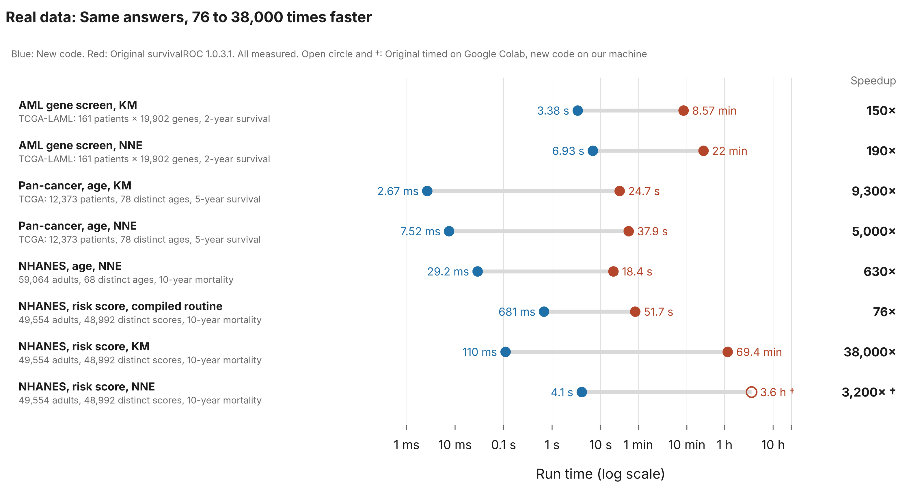
AML marker screen (TCGA-LAML). 161 patients with acute myeloid leukaemia, 103 deaths, and RNA-seq for 19,902 expressed genes. For each gene we computed the AUC for overall survival at 2 years. This is the “screen every marker” use.
- KM method: 514 seconds with the original, 3.4 seconds with the new code (150×).
- NNE method: 1,323 seconds against 6.9 seconds (190×).
- All 19,902 genes returned identical output for both methods.
The gain is modest here because each call is on 161 patients, where the original is at its best.
Pan-cancer cohort (TCGA). 12,373 patients across 33 tumour types, 4,139 deaths, with age at diagnosis as the marker and 5-year overall survival as the outcome.
- KM method: 24.7 seconds against 0.003 seconds (about 9,300×).
- NNE method: 37.9 seconds against 0.008 seconds (about 5,000×).
- Output identical.
Age in whole years has only 78 distinct values, which keeps the original tolerable. A continuous marker on the same cohort is much harder for it, as the next section shows.
NbClust data
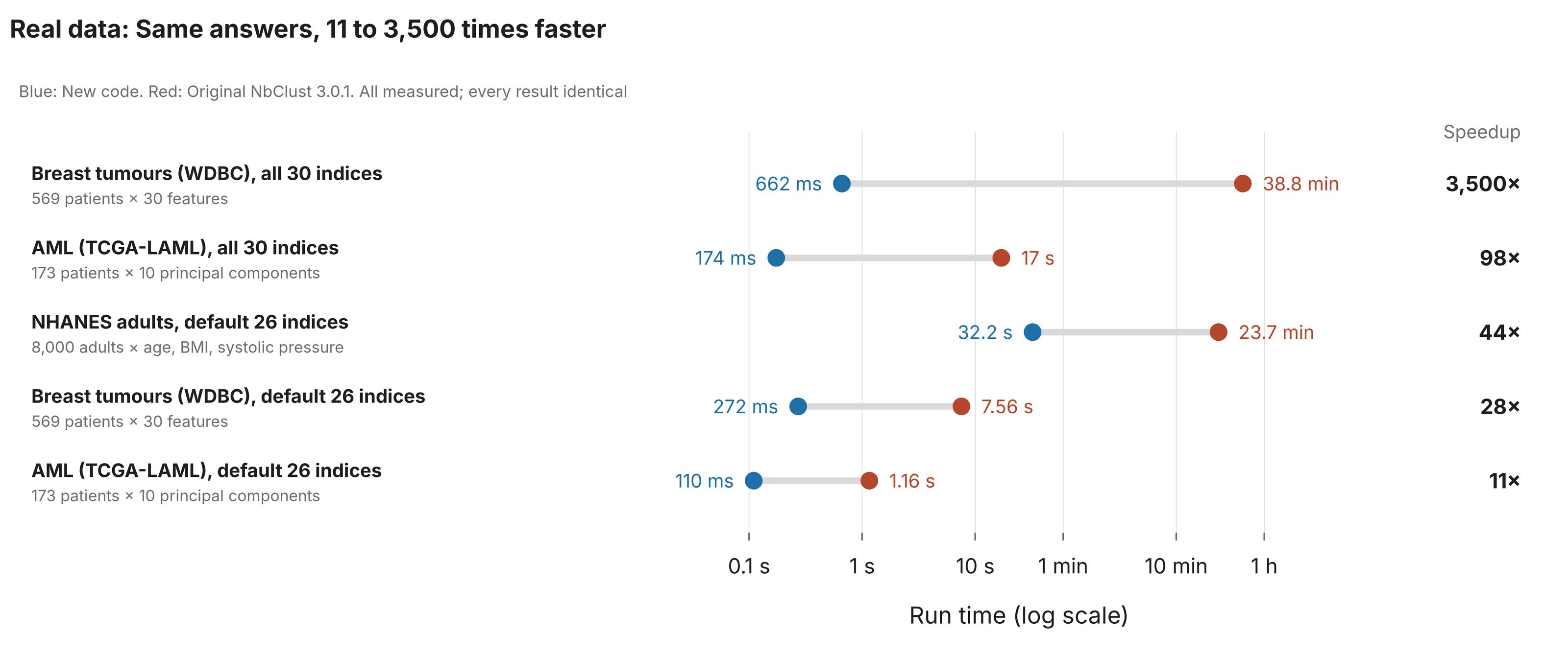
Breast tumours (Wisconsin Diagnostic Breast Cancer). 569 patients, 30 measurements of cell nuclei from fine-needle aspirates. This is a classic clustering benchmark.
- All 30 indices: 38.8 minutes with the original, 0.66 seconds with the new code (3,500×).
- Default 26 indices: 7.6 seconds against 0.27 seconds (28×).
AML (TCGA-LAML). 173 patients, clustered on the first 10 principal components of the 1,000 most variable genes.
- All 30 indices: 17.0 seconds against 0.17 seconds (98×).
- Default 26 indices: 1.16 seconds against 0.11 seconds (11×).
NHANES adults. 8,000 US adults, clustered on age, body-mass index and systolic blood pressure.
- Default 26 indices: 23.7 minutes against 32 seconds (44×).
Every one of these returned identical output. The gain is largest where the fourth-power term dominates and smallest on the 173-patient cohort in default mode, where the original is already quick.
Replication
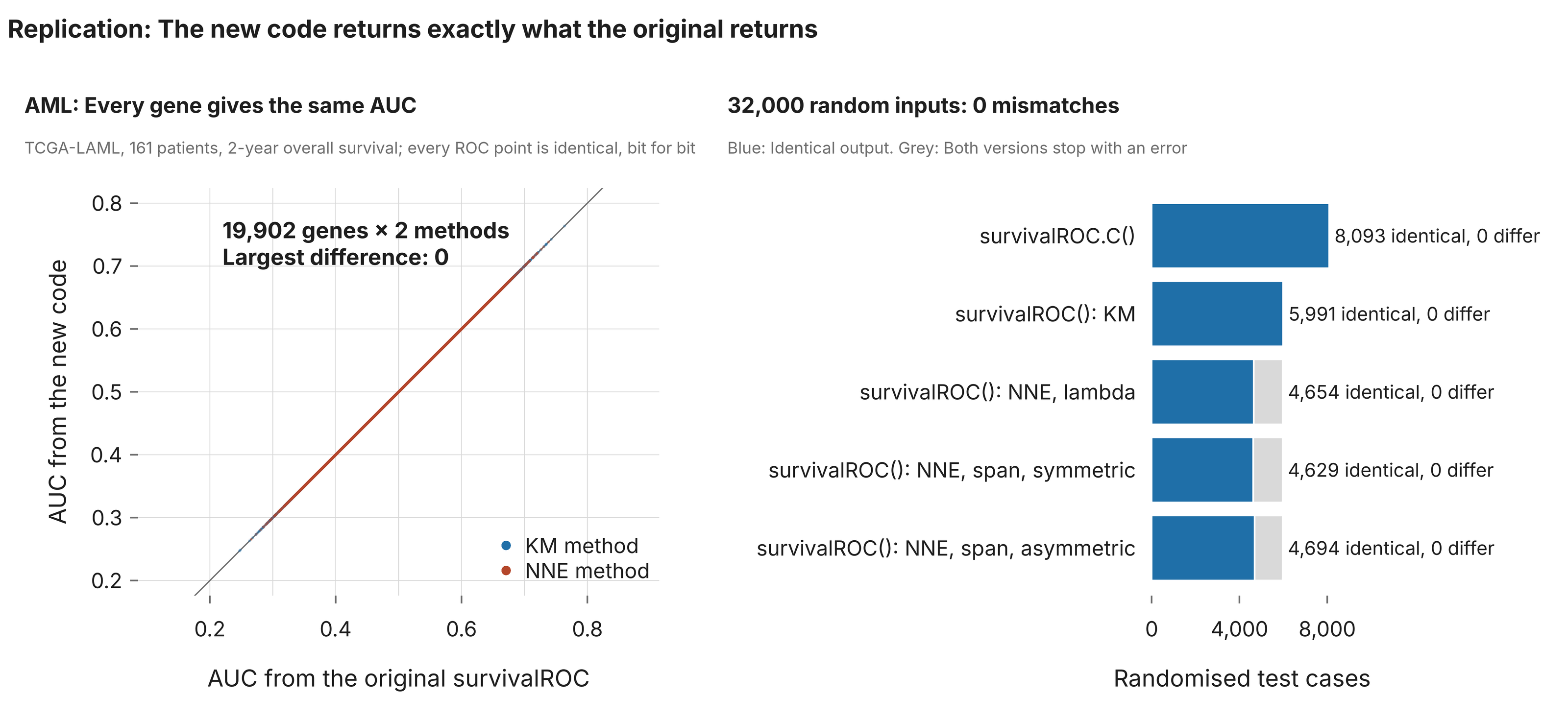
survivalROC. We generated 32,000 random inputs covering tied times, tied markers, heavy and light censoring, missing values, entry times, custom cut-offs and every method and option. The new code returned identical output in 28,061 cases. In the other 3,939, both versions stopped with an error, because the input had no event before the time point. There were no mismatches. A further 150 random inputs with 3,000 to 60,000 patients were also identical.
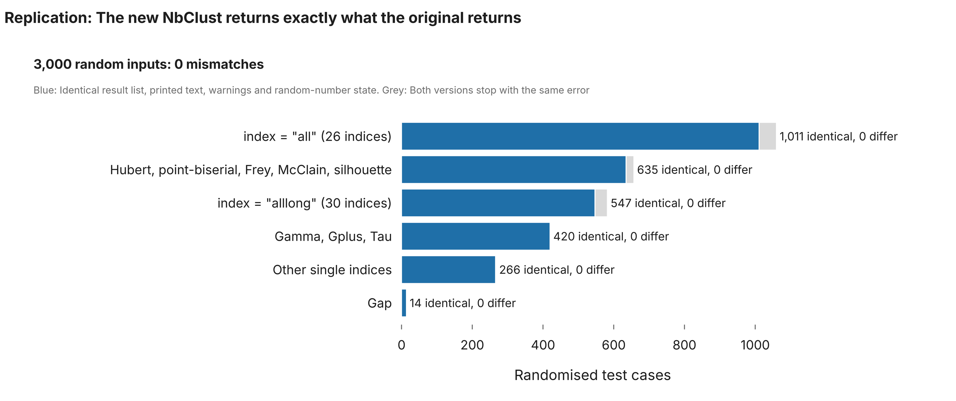
NbClust. We generated 3,000 random inputs across all nine clustering methods, six distance measures, every index on its own and both combined modes, with tied values, duplicated points, missing values and user-supplied dissimilarities. The new code matched the original in 2,893 cases on four things at once: The result, the printed text, the warnings and the state of the random-number generator afterwards. In the other 107, both versions stopped with the same error. There were no mismatches.
Two problems surfaced during NbClust testing, and both were ours. The first test harness reset its own random seed and quietly ran the same two cases 300 times. And one case in 1,500 gave identical results with fewer warnings, because a cached value warned once where the original warned seven times. Both were fixed before the final run.
Simulated data
Simulated data let us push the size while keeping everything else fixed.
survivalROC. Continuous marker, continuous times, about 60% events.
| Patients | Function | Original | New | Speedup |
|---|---|---|---|---|
| 1,000 | survivalROC(), KM | 9.7 s | 0.0007 s | 13,000× |
| 1,000 | survivalROC(), NNE | 23.1 s | 0.003 s | 7,400× |
| 5,000 | survivalROC(), KM | 16 min | 0.009 s | 110,000× |
| 5,000 | survivalROC(), NNE | 42 min | 0.05 s | 50,000× |
| 5,000 | survivalROC.C() | 6.3 s | 0.012 s | 530× |
| 20,000 | survivalROC.C() | 4.9 min | 0.17 s | 1,800× |
| 100,000 | survivalROC(), KM | not run | 2.9 s | |
| 100,000 | survivalROC(), NNE | not run | 18 s | |
| 100,000 | survivalROC.C() | not run | 3.4 s |
The speedup is not a fixed number. It grows with the cohort, because the two versions follow different growth curves.
NbClust. Four Gaussian clusters in 10 dimensions.
| Observations | Indices | Original | New | Speedup |
|---|---|---|---|---|
| 100 | All 30 | 2.3 s | 0.12 s | 19× |
| 200 | All 30 | 25.9 s | 0.17 s | 157× |
| 300 | All 30 | 127 s | 0.20 s | 620× |
| 400 | All 30 | 386 s | 0.29 s | 1,350× |
| 500 | All 30 | 992 s | 0.34 s | 2,900× |
| 500 | Default 26 | 3.2 s | 0.19 s | 16× |
| 1,000 | Default 26 | 13.7 s | 0.47 s | 29× |
| 2,000 | Default 26 | 55.7 s | 1.8 s | 31× |
| 4,000 | Default 26 | 225 s | 7.0 s | 32× |
With all 30 indices, the ratio keeps climbing with the data. With the default 26, it settles near 30, because both versions grow at the same rate and what remains in the new code is mostly R’s own arithmetic over the distance matrix.
The largest datasets we could compute
survivalROC: 49,554 adults
The largest public cohort with individual survival times that we could reach was NHANES with linked mortality: Ten cycles of the US National Health and Nutrition Examination Survey (1999 to 2018), with deaths followed through the National Death Index to the end of 2019.
- 59,064 adults were eligible for mortality follow-up, and 9,249 died.
- 49,554 of them had age, sex, body-mass index and systolic blood pressure recorded, with 6,822 deaths.
- For those we built a simple risk score with a Cox model, which gives 48,992 distinct marker values. The outcome was death within 10 years.
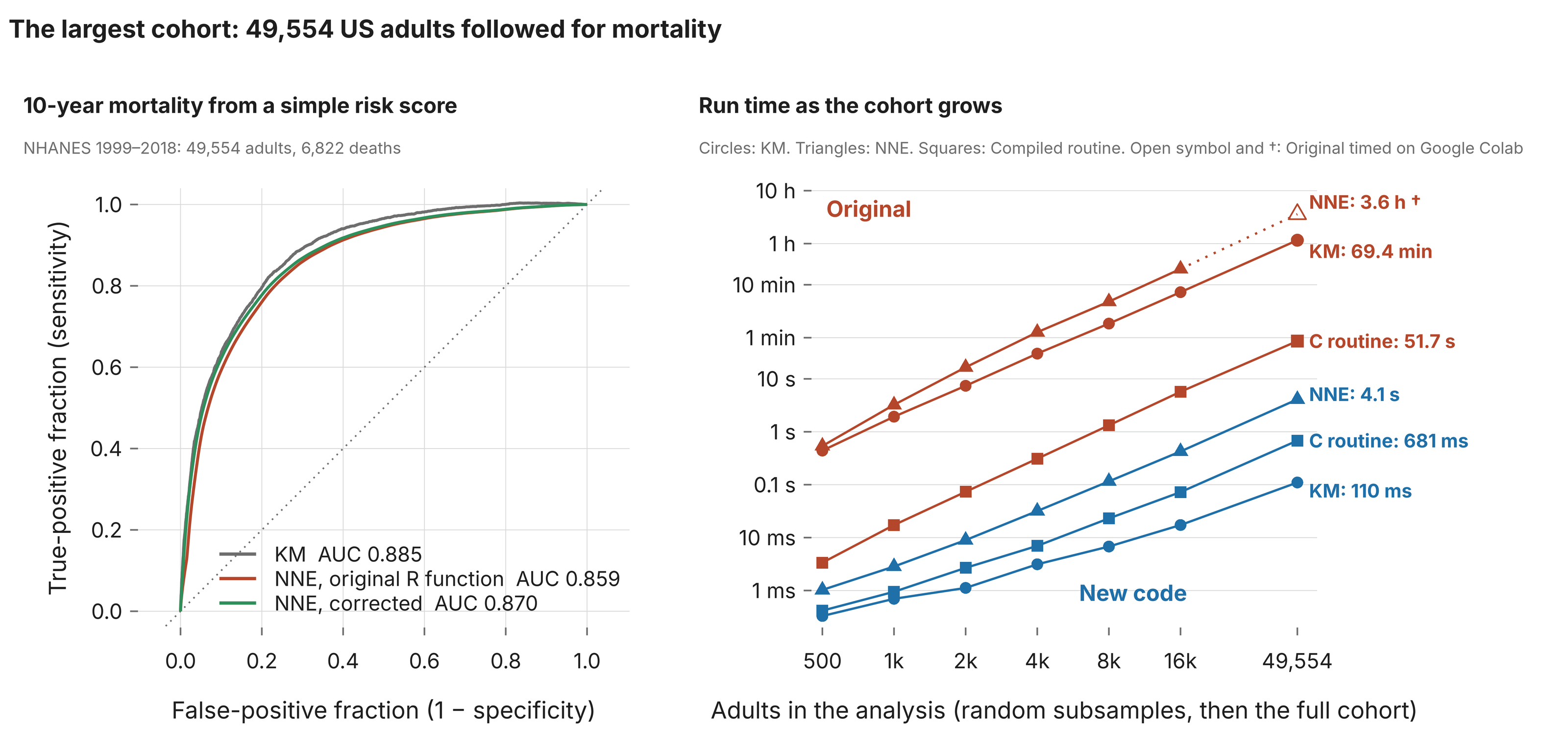
On the 49,554-adult cohort with the risk score:
- KM method. 69 minutes (4,166 seconds) with the original, 0.11 seconds with the new code. That is 38,000×, with identical output at all 48,993 points of the curve.
- Compiled routine. 51.7 seconds with the original, 0.68 seconds with the new code (76×), identical output.
- NNE method. 3.6 hours (12,947 seconds) with the original, 4.1 seconds with the new code. The original was timed on a Google Colab CPU and the new code on our machine, so the ratio of about 3,200× compares two computers and is approximate. On one machine, the 16,000-adult subsample took the original 1,195 seconds and the new code 0.43 seconds (2,800×), with identical output. At full size we also ran both versions on our machine with the score rounded to two decimals (665 distinct values): 151 seconds against 0.07 seconds, identical output.
On all 59,064 adults with age as the marker, the NNE method took 18.4 seconds with the original and 0.029 seconds with the new code (630×), identical output.
One difference that only this run exposed. The first full-cohort comparison was not identical. Thirteen of the 48,993 points on the KM curve differed in the last binary digit, a relative difference of 2 × 10⁻¹⁶. The cause was one line: The original takes the mean() of a TRUE/FALSE vector, and R computes that quotient in extended precision before rounding, which is not always the same number as the count divided by n. It never differs at 161, 5,000 or 16,000 patients. It sometimes differs at 12,373 and 49,554. The new code now divides the way R does, and every comparison in this post was re-run after that change. The 32,000 small random tests had not caught it, which is why the large-cohort tests exist.
Two things about this cohort are worth stating plainly. Follow-up is recorded in whole months, so there are only 250 distinct times, and that makes the original’s work lighter than in the simulations. And the risk score was fitted on the same people it is evaluated on, so the AUC of 0.87 to 0.89 is optimistic. The score is there to give the software a realistic continuous marker, not to propose a model.
NbClust: 8,000 adults
The limit for NbClust is memory, not time. Every index is built on the full matrix of pairwise distances, and the original keeps several copies of it.
The largest run we completed with both versions was the 8,000-adult NHANES cohort in the default mode: 1,420 seconds with the original, 32 seconds with the new code, identical output.
For the 30-index mode, the largest dataset on which we ran both versions was the 569-patient tumour set above. The new code on its own goes much further. On the same 8,000 adults it computed all 30 indices in 97 seconds. We did not run the original at that size: It needed 16.5 minutes for 500 observations, and its cost grows with the fourth power.
Bugs in the originals
Matching a program exactly means reading all of it, and both packages had behaviours that stood out. In both new packages, the default mode reproduces the original exactly, defects included, because bit-identity demands it. A new argument, corrected = TRUE, fixes them.
survivalROC
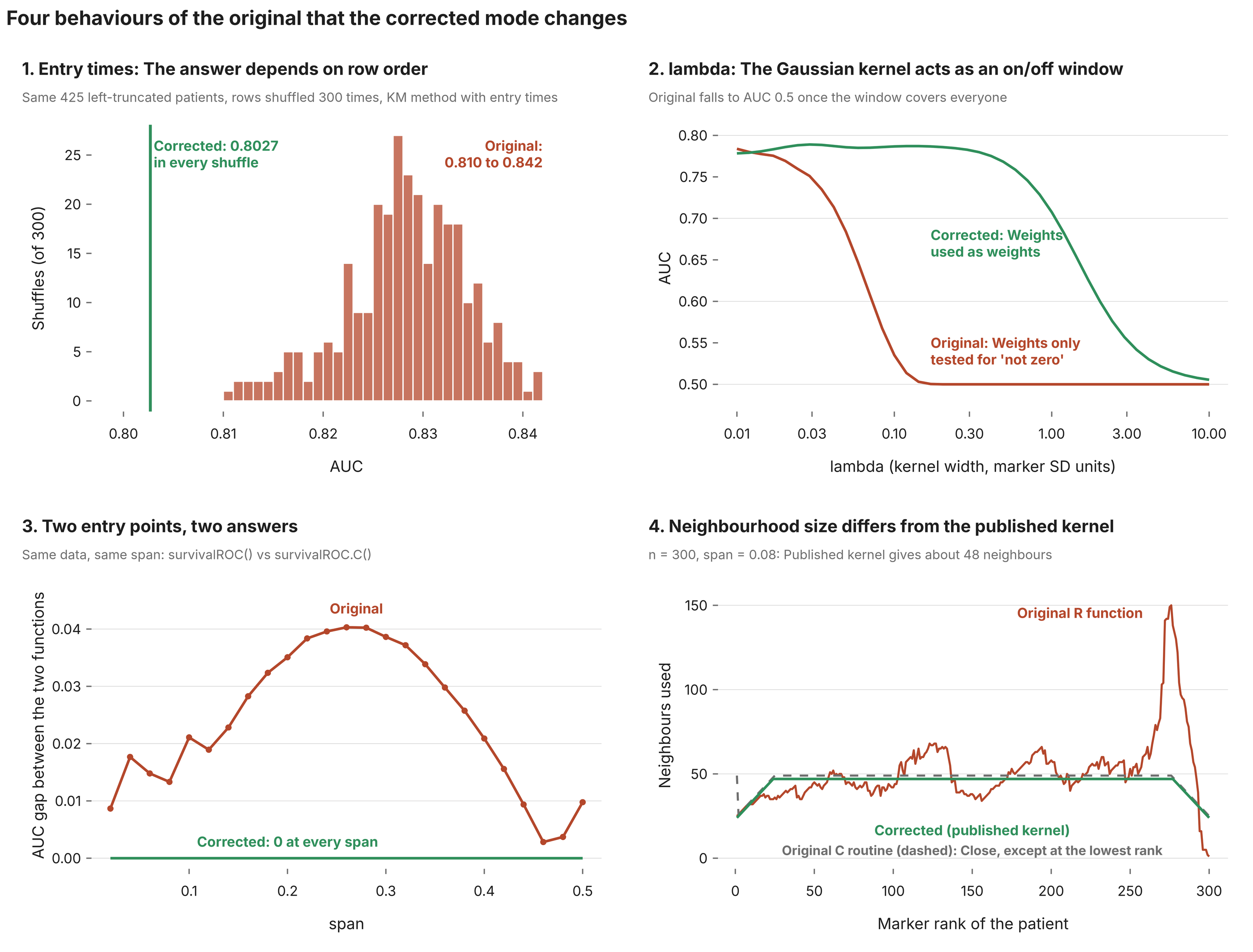
| # | Defect in survivalROC 1.0.3.1 | Effect | Fix in corrected = TRUE |
|---|---|---|---|
| 1 | Entry times are not sorted with the data. The function sorts time, status and marker by time, but leaves entry in its input order. | With left-truncated data the result depends on the order of the rows. On 425 simulated patients, 300 shuffles of the same rows gave AUCs from 0.810 to 0.842. The value with the columns aligned is 0.803. | entry is sorted with the other columns. The result no longer changes with row order, and it matches the original whenever the input happens to be sorted by time already. |
| 2 | The lambda kernel is not used as a weight. The code computes Gaussian weights and then combines them with a logical “and”, which only asks whether each weight is non-zero. | The smooth kernel becomes a hard window about 27 × lambda wide on each side. Once that window covers everyone, the AUC is exactly 0.5. | The weights are used as weights in a weighted Kaplan-Meier estimate. |
| 3 | survivalROC() and survivalROC.C() disagree. Given the same data and span, the R function and the compiled routine build different neighbourhoods. | Two answers for one estimator. The AUC gap reached 0.04 in simulation and was 0.010 on NHANES (0.859 against 0.870). | Both entry points use the kernel as published: A patient is a neighbour if the empirical distribution of the marker differs by less than the span. They now return the same curve. |
| 4 | Neighbourhood size drifts from the published kernel. In the R function the lower side of the window is set by marker distance, not by rank, and a computed index is never used. In the C routine the window for the smallest marker value is centred in the middle of the sample. | The number of neighbours varies from near 0 to three times the intended number across the marker range. | The published kernel gives a constant number of neighbours away from the edges. |
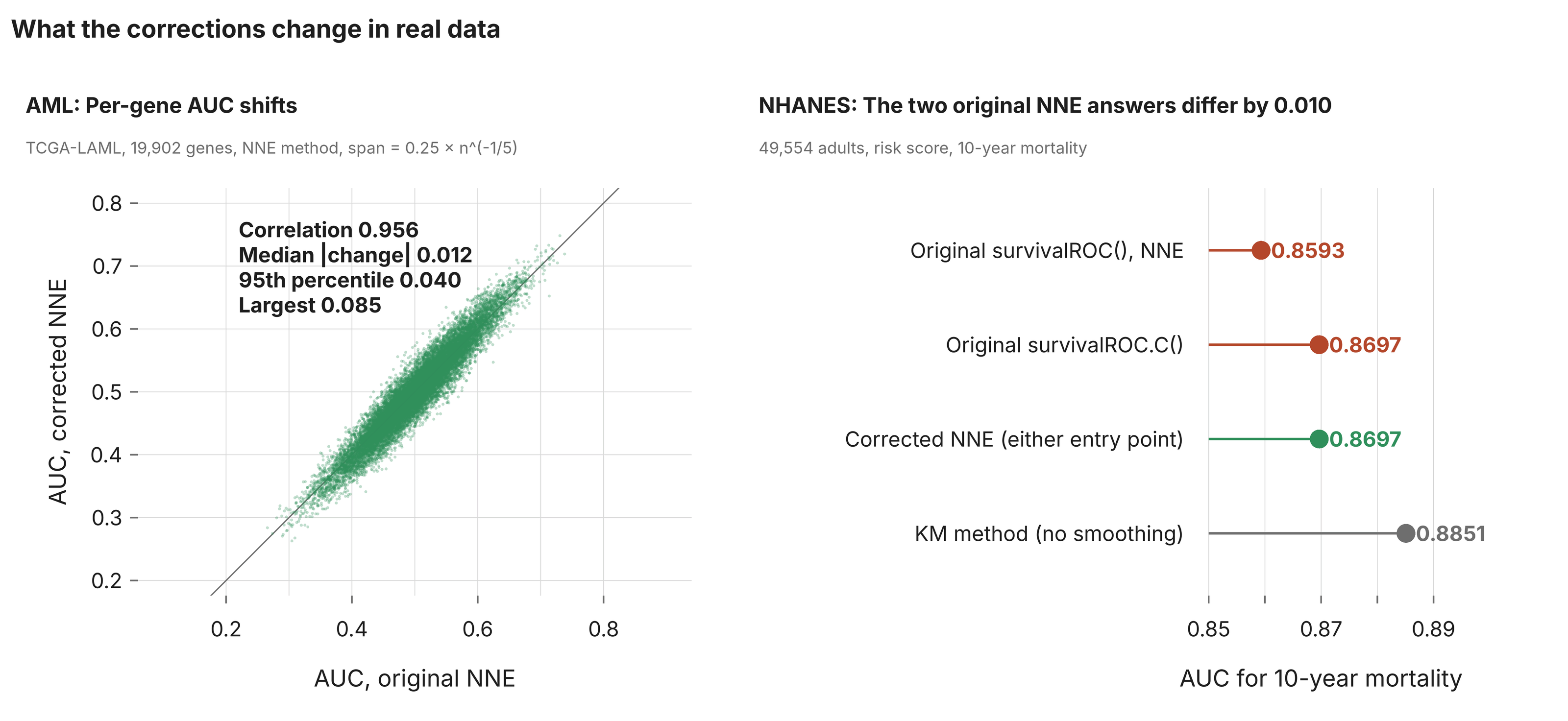
How much do the corrections matter in practice?
- On NHANES, the corrected NNE estimate is 0.8697, the same to four decimals as the original compiled routine. The original R function gives 0.8593.
- On the AML screen, per-gene AUCs from the original and the corrected NNE correlate at 0.956. The median change is 0.012, 1 gene in 20 moves by more than 0.040, and the largest change is 0.085. That is enough to reorder a ranked list of candidate markers.
- Defect 1 only affects analyses that pass
entry. Most published uses do not.
We validated the corrected mode separately. It agrees with a slow reference written directly from the published formulas to 8 × 10⁻¹⁶ over 400 random inputs, and it gives the same result for any row order.
NbClust
The gap statistic (Tibshirani, Walther and Hastie, 2001) compares how tightly the data cluster with how tightly structureless data would cluster. The structureless data are simulated: Draw points uniformly over the range of each variable, several times, and average. NbClust draws 10 such reference sets.
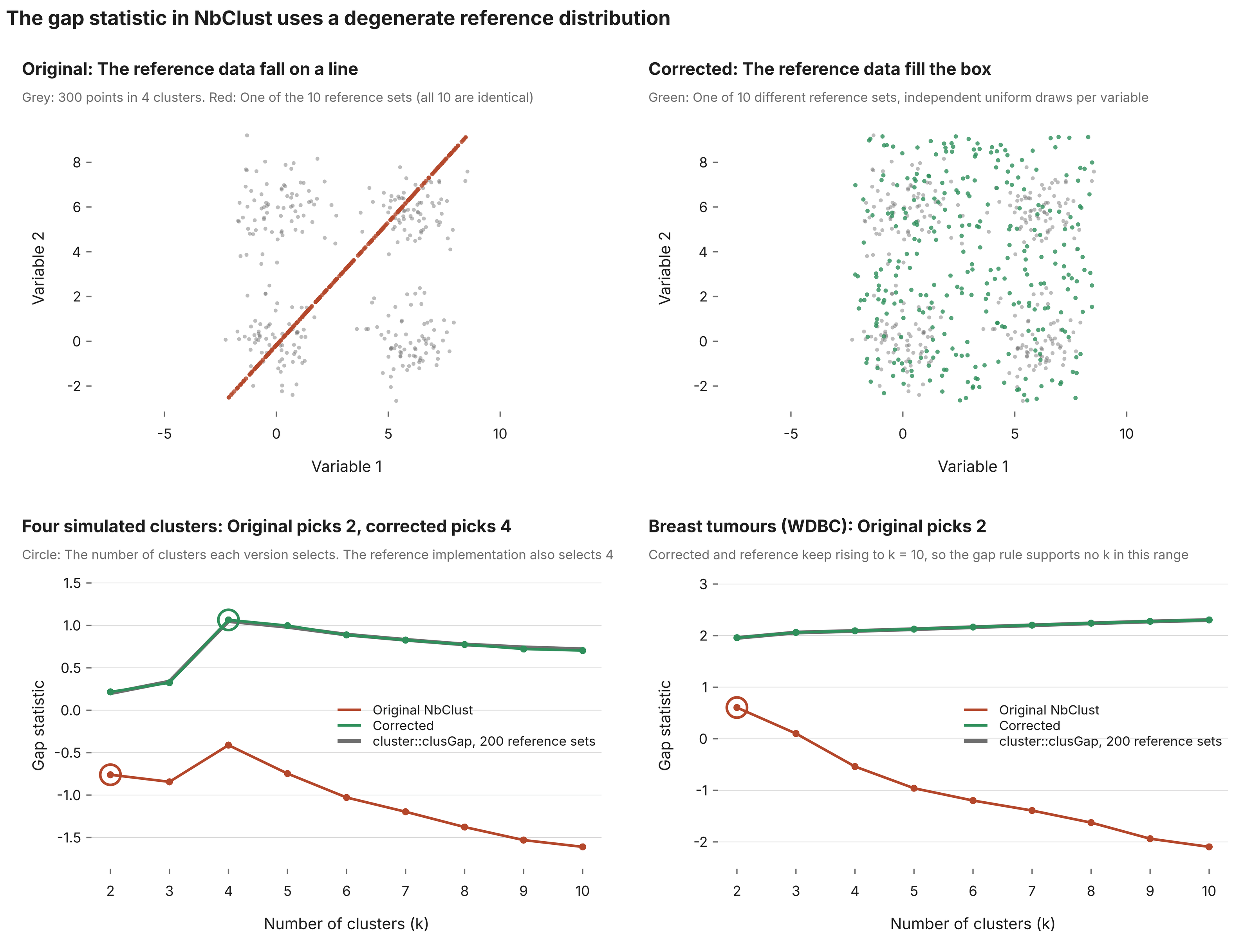
| # | Defect in NbClust 3.0.1 | Effect | Fix in corrected = TRUE |
|---|---|---|---|
| 1 | The reference data are not random across variables. The function that simulates one variable resets the random seed to 1 every time it is called. | Every variable receives the same sequence of uniform numbers, rescaled to its own range. The correlation between any two reference variables is exactly 1, so the reference points lie on a straight line and not in a box. | Each variable gets its own independent uniform draws. |
| 2 | The 10 reference sets are one set. The same seed reset applies to every replicate. | All 10 replicates are identical. The Monte Carlo average is an average of one draw, and its reported spread is an artefact of defect 3. | The 10 reference sets are 10 different draws, made once per call and reused for every number of clusters. |
| 3 | Replicates are weighted inconsistently. The first replicate weights each cluster by its size minus one, the other nine by its size. A one-member cluster is passed to var() as a plain vector, which returns the variance across its variables. | The dispersion of the first replicate is not comparable with the rest. | Every replicate uses the same pooled within-cluster dispersion. A one-member cluster contributes zero. |
| 4 | The caller’s random numbers are overwritten. NbClust() calls set.seed(1) internally for k-means and for the gap. | Any random step that follows a call to NbClust in the same script starts from seed 1, whatever seed the user set. | The random-number state is saved on entry and restored on exit. |
| 5 | No answer is not handled. If no number of clusters in the range meets the gap rule, the variable holding the answer is never assigned. | With index = "gap" the function would stop with an internal error. We reached this path only with the corrected gap; the original’s flawed reference met the rule in all 60 random datasets we tried. | The gap’s preferred number is reported as missing, with a warning that says why. |
How much does this matter?
- On simulated data with four well-separated clusters, the original gap statistic picks 2. The corrected version picks 4. So does
cluster::clusGap, the standard implementation, run with 200 reference sets. - On the tumour dataset, the original picks 2. The corrected gap and
clusGapboth rise steadily to 10 clusters, which means the gap rule supports no number in the range. The corrected mode reports that instead of a number. - The other 29 indices are untouched. On the tumour dataset the majority vote is 2 clusters with or without the correction, because the gap is one vote in 30.
- The cost is negligible. The corrected 30-index run on the tumour dataset took 0.77 seconds.
The corrected gap curves agree with clusGap closely on all three datasets we tried, and with an independent implementation of the published formula to the four decimals NbClust reports.
The fixes in both packages are our reading of the published methods. They have not been reviewed by the packages’ authors.
How to reproduce this
The source, the tests and the benchmark scripts for each package are in one bundle:
- survivalROCfast: survivalROCfast_bundle.tar.gz
- NbClustFast: NbClustFast_bundle.tar.gz
You need R (4.0 or later for survivalROCfast, 3.1 or later for NbClustFast) and a C compiler.
survivalROCfast
tar -xzf survivalROCfast_bundle.tar.gz
cd survivalROCfast_bundle
bash run_all.sh
run_all.sh installs the CRAN survivalROC and the new package, runs 5,000 randomised identity checks, tests the corrected mode against a slow reference, and prints a timing table of old against new. Add a number to also time the original’s R code at that size, for example bash run_all.sh 5000 (about an hour).
To use it in your own analysis:
library(survivalROCfast)   # in place of library(survivalROC)

roc <- survivalROC(Stime = time, status = event, marker = score,
                   predict.time = 365 * 3, method = "KM")
roc$AUC

# the corrected estimators
roc2 <- survivalROC(Stime = time, status = event, marker = score,
                    predict.time = 365 * 3, method = "NNE",
                    span = 0.25 * length(time)^(-0.2), corrected = TRUE)
The other scripts in the bundle rebuild each analysis from public data:
get_data.shdownloads the public data: TCGA-LAML and the Pan-Cancer Atlas survival table from UCSC Xena, and the NHANES files with linked mortality from the CDC.demo_aml.Rruns the AML gene screen anddemo_pancan.Rthe pan-cancer comparison.prep_nhanes.Rbuilds the NHANES cohort andnhanes_run.Rtimes one method on it.test_equiv.R,test_large.Randtest_corrected.Rare the identity tests and the correction tests.figures_src/holds the scripts and the result tables behind every survivalROC figure in this post.
The package is licensed GPL (≥ 2), the same as the original, because it carries a verbatim copy of the original R function as its fallback.
NbClustFast
tar -xzf NbClustFast_bundle.tar.gz
cd NbClustFast_bundle
bash run_all.sh
run_all.sh installs the CRAN NbClust and the new package, runs 400 randomised identity checks, tests the corrected mode, and prints a timing table of old against new. Add a number to time the original’s 30-index mode up to that size, for example bash run_all.sh 500 (about 25 minutes).
To use it in your own analysis:
library(NbClustFast)   # in place of library(NbClust)

res <- NbClust(data = x, distance = "euclidean", min.nc = 2, max.nc = 10,
               method = "ward.D2", index = "alllong")
res$Best.nc

# the corrected gap statistic, with your random seed left alone
res2 <- NbClust(data = x, distance = "euclidean", min.nc = 2, max.nc = 10,
                method = "ward.D2", index = "alllong", corrected = TRUE)
The other files in the bundle:
test_equiv.Randtest_corrected.Rare the identity tests and the correction tests.bench.Randreal.Rtime one configuration on simulated and real data, andverify.Rchecks that saved results from the two versions are identical.build_from_source/holds the script that derives the package from the CRAN source, so every change to the original is visible in one place.figures_src/holds the scripts and the result tables behind every NbClust figure in this post.
The package is licensed GPL-2, the same as the original, whose source it contains.
Methods in brief
- Baselines: survivalROC 1.0.3.1 and NbClust 3.0.1 (CRAN), R 4.5, Linux, 4 cores, all code single-threaded.
- Timing: Elapsed time of one call. For survivalROC, calls under 0.3 seconds were repeated and averaged, and full-cohort NHANES timings of the new code are the median of five runs. For NbClust, printed output was captured and plots were sent to a null device.
- Identity:
identical()on the complete returned list, plus identical printed messages. The NbClust random tests also compared warning messages and the next random number drawn after the call. - survivalROC random tests: 32,000 inputs, 2 to 300 patients, with continuous and discrete markers, tied and untied times, 0 to 100% events, missing values, entry times and custom cut-offs. A further 150 inputs with 3,000 to 60,000 patients, using few cut-offs or few marker values so that the original stays affordable.
- NbClust random tests: 3,000 inputs, 12 to 120 observations, 2 to 6 variables, 9 clustering methods, 6 distances, each index alone and both combined modes. NbClust settings were Ward linkage (
ward.D2), Euclidean distance and 2 to 10 clusters, unless a test varied them. - AML (survivalROC): TCGA-LAML RNA-seq (HiSeqV2) and curated survival from UCSC Xena; genes with zero variance removed; prediction time 730 days.
- Pan-cancer: TCGA Pan-Cancer Atlas clinical table from UCSC Xena; overall survival; prediction time 1,825 days.
- NHANES (survivalROC): Continuous NHANES 1999 to 2018, adults aged 18 and over, public-use linked mortality files (follow-up to 31 December 2019); follow-up in months from the examination; prediction time 120 months; risk score from a Cox model on age, sex, BMI (linear and squared) and systolic blood pressure.
- Tumour data (NbClust): Wisconsin Diagnostic Breast Cancer from the UCI Machine Learning Repository; 30 features, standardised.
- AML (NbClust): TCGA-LAML RNA-seq from UCSC Xena; 1,000 most variable genes, first 10 principal components, standardised.
- NHANES (NbClust): A random 8,000 of the 49,554 adults described above; age, BMI and systolic pressure, standardised.
- Simulations: For survivalROC, standard normal marker, exponential event times with hazard exp(marker), independent exponential censoring, prediction time 1. For NbClust, four Gaussian clusters in 10 dimensions with random centres.
- Gap reference:
cluster::clusGapwith 200 reference sets, squared Euclidean dispersion, uniform reference over the original variable ranges, the same Ward clustering, and the Tibshirani selection rule. - References: Heagerty PJ, Lumley T, Pepe MS. Time-dependent ROC curves for censored survival data and a diagnostic marker. Biometrics 2000;56:337–344. Charrad M, Ghazzali N, Boiteau V, Niknafs A. NbClust: An R package for determining the relevant number of clusters in a data set. J Stat Softw 2014;61(6). Tibshirani R, Walther G, Hastie T. Estimating the number of clusters in a data set via the gap statistic. J R Stat Soc B 2001;63:411–423.
Comments